Social media data for better local forecasts

 https://github.com/4castRenewables/climetlab-plugin-a2
The data is available via the S3 buckets at ECMWF and can be downloaded using the CliMetLab

climetlab-maelstrom-social-media plugin

We directly provide the precipitation data used in this study. In compliance with Twitter terms of service restrictions the Tweets will not be shared in a public repository instead the Tweet IDs are available in the repository. The code of the application is provided on the 4Cast GitHub account and instructions for usage are provided.

This application is being delivered by 4cast.

With this app, we aim to use data provided by social media as weather sensors. As a first step, we use texts of Tweets to predict the occurrence of rain (“raining”, “not raining”) at the Tweet’s location and time of creation.

We use historical tweets from the years 2017-2020 that include keywords related to the presence of rain, e.g., “rain”, “sunny” or “drizzle.” Locations need to be attached to these tweets such that we can assign weather data to them. Locations can be assigned to Tweets in two ways. The user may opt in to be tracked by Twitter such that GPS data are assigned to every tweet of the location of the user. Alternatively, users can tag their tweets from a curated list of locations by Twitter. We use Tweets with locations from either method. However, we exclude tweets that are tagged with a location that surface area is greater than 100 square kilometres, which corresponds to the spatial resolution of our weather data. Here, we focus on tweets in the English language that originate from any location within the United Kingdom. This allows us to resort to the most popular pretrained models in natural language processing (NLP), which are usually trained in English. In total, our dataset includes 1.3 million Tweets, 1 million of which have a tagged location and 300k have GPS coordinates attached. 700k Tweets are tagged “not raining” while 600k Tweets are tagged “raining”.

Precipitation data are taken from the ECMWF-IFS weather forecasting model during the years of 2017-2020. The model has a spatial resolution of 0.1° in both horizontal and vertical directions and a temporal resolution of 1h. Precipitation above the noise level of the data is interpreted as “raining” by our model. We assign Tweets precipitation values based on the nearest data point in both space and time. We plan to study the impact of any form of averaging for this assignment in the future.

To improve the results, texts are preprocessed to match vocabulary of the model and the input as well as focusing the model’s attention on the relevant parts of the text. We remove the hyperlinks and hashtags (unless they represent a keyword) and rephrase colloquial terms. If emojis are directly related to precipitation, e.g. umbrella, rain cloud …, these emojis are converted to text. Remaining emojis are removed from the text. For training, we only retain texts that still contain at least one keyword after preprocessing. In addition, we remove all Tweets that contain the word “Sun” (note, capital “S”), as this word appears to be mostly used when referring to the British newspaper “The Sun” or referring to Sunday, which means that these Tweets usually contain insufficient information for our prediction task.

For Experiment 1, we only use a subset of our dataset, which corresponds to all Tweets posted in 2020. This allows us to assess the relevance of training set size. For the second Experiment, we use our full dataset. We use 80% of our datasets for training and withhold 20% for testing.

We use cross entropy as our loss function. The proficiency of the model is evaluated via the f1 score of the minority class (“not raining”). The f1 score is the harmonic mean of the precision and recall.

Generally, our problem can be phrased as a text classification task, where deep learning models based on the transformer architecture (Vaswani et al., 2017) achieve state-of-the-art results (e.g. Yang et al., 2019). Transformers use self-attention to attribute varying relevance to different parts of the text. Based on transformers the BERT model was developed (Devlin et al., 2019), which includes crucial pretraining steps to familiarise the model with relevant vocabulary and semantics. In addition, the DeBERTa model (He et al., 2021a) adds additional pre-training steps and disentangles how positional and text information is stored in the model to improve performance. For this experiment we rely on the most recent version of the model, which is DeBERTaV3 (He et al., 2021b).

We use the default version of DeBERTaV3_small as described in He et al., 2021b, with an adopted head for text classification. For this, we add a dropout layer with user-specified dropout rate and a pooling layer that passes the embedding of the special initial token ([CLS], comprising the meaning of the whole Tweet) to the loss function.

We initialise the model with pre-trained weights as explained in He et al., 2021b. We then employ a lower learning rate compared to the pre-training step to train the full model with our small dataset, which only contains Tweets posted in 2020. For both our experiments, we use default parameters as given in He et al., 2021b. For hyper-parameters, we use parameters as listed in their Table 10. After hyper-parameter tuning, we only deviate in the following parameters that we use for both our experiments, where our batch size is 32, learning rate is 3e-5, drop out of the task layer is 0.1, weight decay is 0.01, training epochs is 1 and the warm up ratio is 0.45. Our best model achieves a f1 score of the minority class (“raining”) of 0.64.

To analyse our results, we use the relative difference between the outputs of the final softmax layer to the respective label as a measure of confidence of the model. First, we focus on tweets labelled as “raining”, where the model predicts “not raining” at a high confidence.

Analogously to Experiment 1, we initialise our weights with pre-trained weights from He et al., 2021b and train with parameters described in Experiment 1. Our best model achieves a f1 score of the minority class of 0.66.

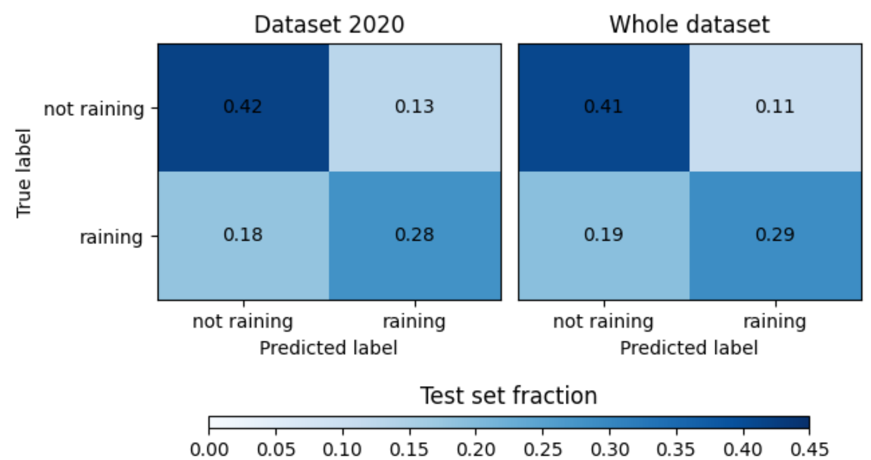
The Figure 3 summarises our results in the form of a normalised confusion matrix. The confusion matrix in the left-panel corresponds to our 2020 dataset (Experiment 1) and the right-hand panel corresponds to the whole dataset.

Our best model achieves an f1 score of the minority class (“raining”) of 0.66 when including all Tweets. The smaller dataset (only Tweets from 2020) achieves a somewhat lower f1 score of the minority class (“raining”) of 0.64. The datasets yield an AUC (Area under the ROC Curve) of 0.77 and 0.76, respectively.

In the future, we aim to use larger model variants and experiment with alternative deep learning models, e.g. XLNet (Yang et al., 2019) or ULMFiT (Howard et al., 2018). In addition, exploring alternative ML techniques like XGBoost (Chen et al., 2016) or the more recent CatBoost (Prokhorenkova et al.,2018) which also allows the user to include embeddings for training.