Neural network emulators for faster forecast models & data assimilation

 https://github.com/ecmwf-projects/infero
Data and code are both provided through the climetlab-maelstrom-radiation repository/pip package. Installation can be done with

pip install climetlab-maelstrom-radiation

Once installed, shell commands to run each of the experiments can be found in the Table 6 below. Note that the first time one of the experiments is run a data download will occur. With a good internet connection this will take ~3 hours and require ~400Gb of disk space. To run the code with a minimal data download (~3Gb), use

--tier 1

below, while noting that the model performance will be dramatically reduced. Details on the location of the data have been documented.
Run commands:

radiation-benchmarks-sw --epochs 50 --batch 512 --model cnn --tier 2
radiation-benchmarks-sw --epochs 50 --batch 512 --model rnn --tier 2
radiation-benchmarks-sw --epochs 50 --batch 512 --model cnn --tier 2 --attention --notf32

This application is being delivered by ECMWF.

This app seeks to emulate the radiative transfer process both for radiation with short and long wavelengths. This is a columnar problem, i.e. sets of inputs & outputs are formed of atmospheric columns, and the task is found within all weather and climate models.

The inputs are profiles of atmospheric state and composition, e.g. temperature and aerosol properties. The inputs either live on model levels (137 levels in the IFS model which is used for the study), model half-levels (138 levels), model interfaces (136 levels) or as scalars. A complete list of the variables can be found in deliverable 1.1 or in the CliMetLab plugin. The CliMetLab provides the inputs gathered by level type, such that 3 input arrays are provided, containing the half-level, full-level & surface variables.

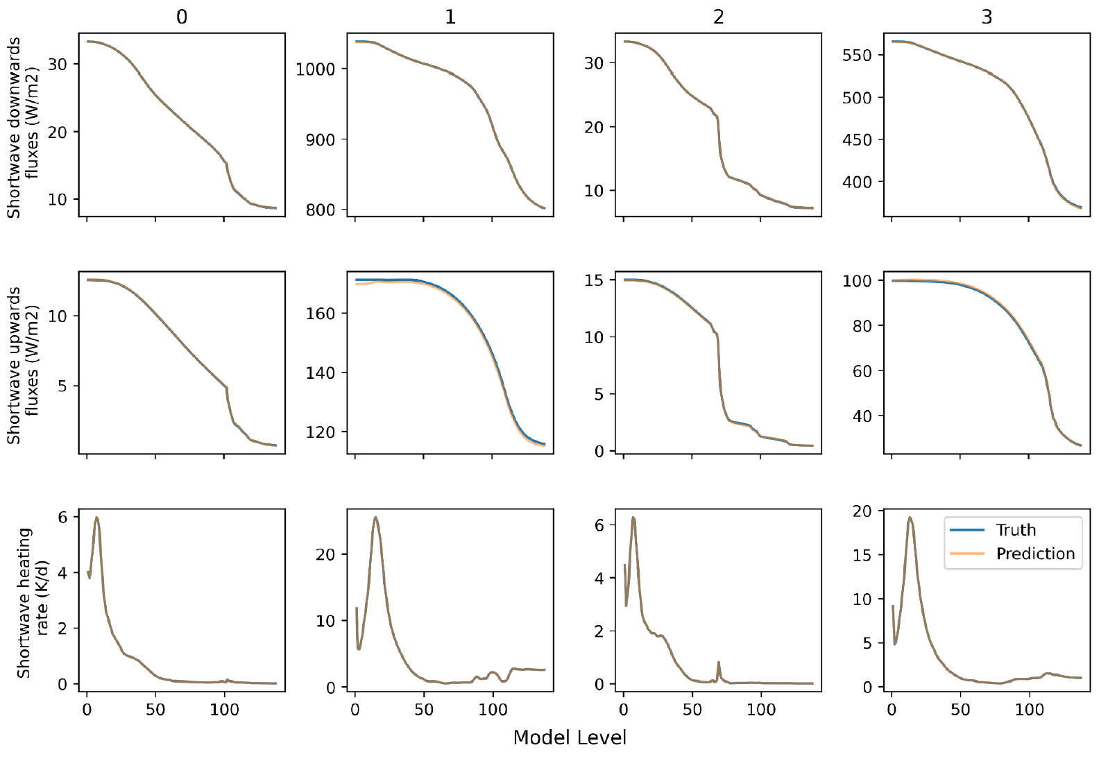
For the outputs, there is a duality between down and up fluxes, the typical output of a conventional scheme, and heating rates. At the surface, fluxes are necessary to heat and cool the surface, in the atmosphere, the heating rates are the desired variable that is used to increment temperature profiles. The two variables are related through

where the left-hand side denotes the heating rate, Fn denotes the net (down minus up) flux, p the pressure, g is the gravitational constant, cp is the specific heat at constant pressure of moist air and i is the vertical index. We will throughout the experiment encode this relationship in a neural network layer and dually learn to minimise errors of the heating rate and flux profiles. Our metrics of interest are therefore the RMSE and MAE of the fluxes and heating rates.

For this phase of reporting, we introduce an extended version of the dataset. This extends the number of example columns used to train the models for learning the radiative transfer process. These can be accessed from the maelstrom-radiation-tf CliMetLab dataset using the subset = “tier-2” argument. This generates a dataset with 21,640,960 examples. This is to be contrasted with the Tier 1 dataset which contained only 67,840 examples. We also introduce Tier 2 subsets for validation and testing, accessible with “tier-2-val” and “tier-2-test”. Each of these contain 407,040 columns from 2019 (training data are taken from 2020). This dataset requires ~400Gb of disk space, a significant amount. We therefore also introduce Tier 3 datasets, which are equivalent for the validation & test splits, but contain “only” 2,984,960 columns, consuming ~60Gb of disk space. We found significant model improvements when using the Tier 2 dataset over the Tier 3 dataset, even when controlling for the number of iterations. Here, we will only present results on the Tier 2 data.

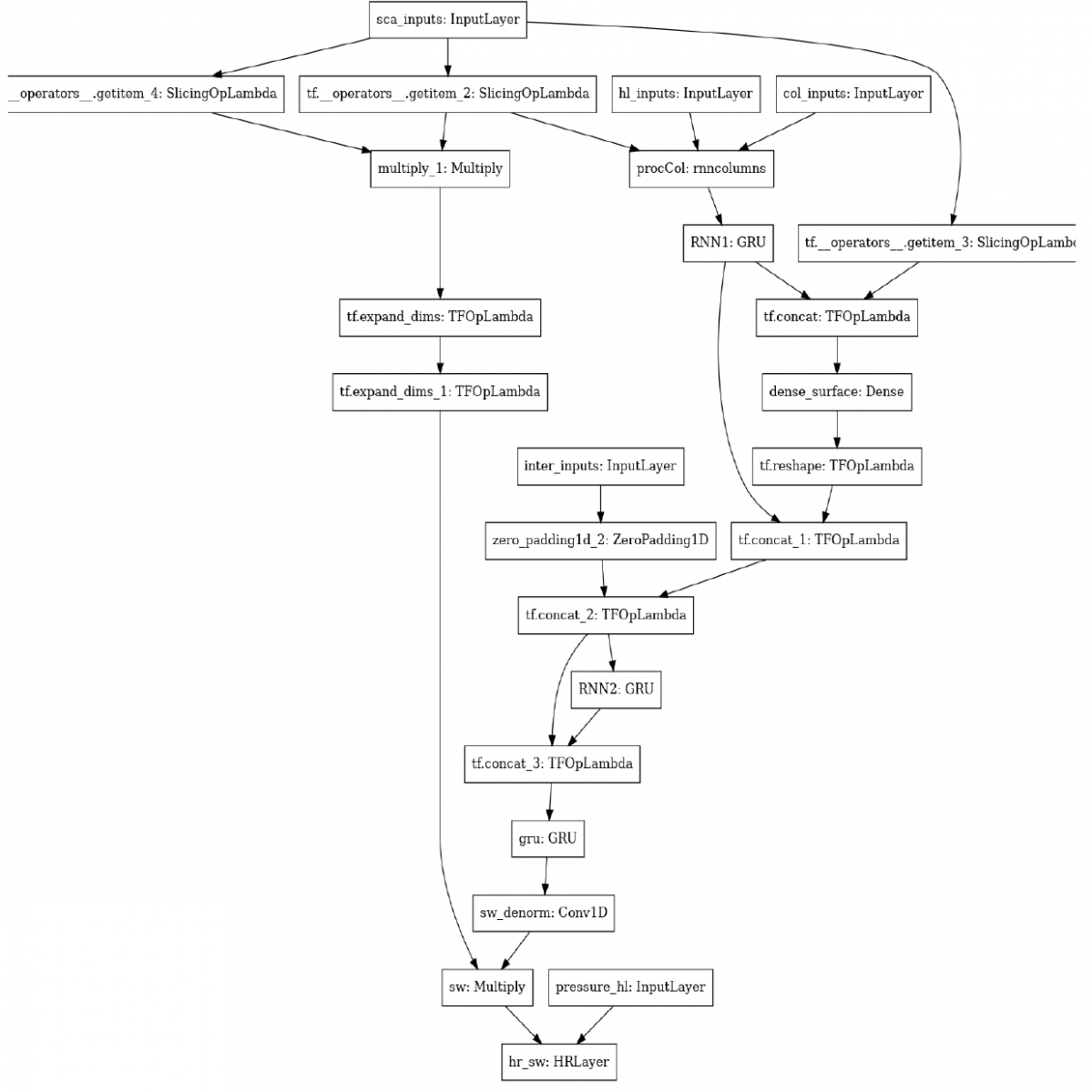
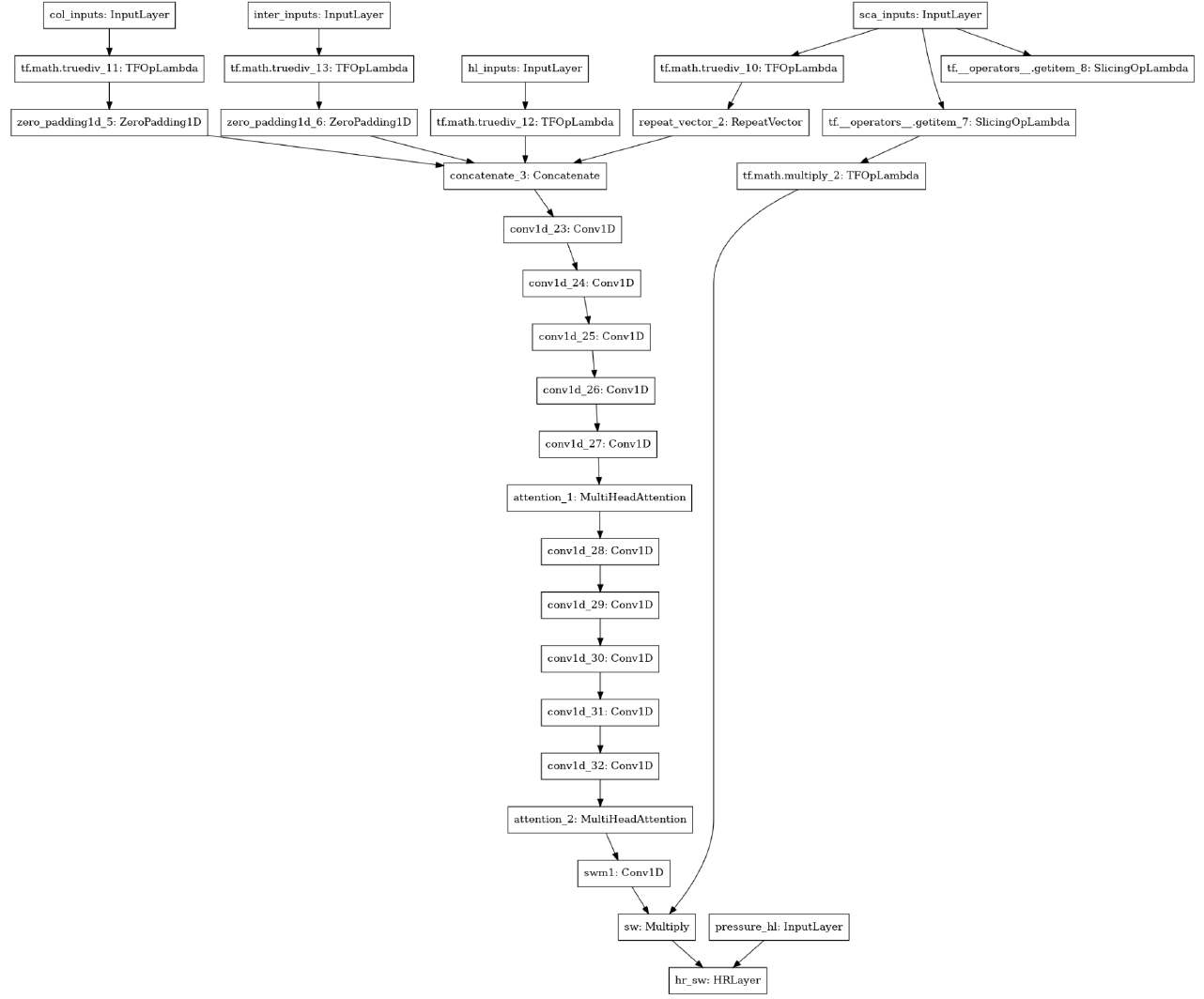
For brevity, we focus our reporting on the shortwave heating process. Equivalent models are being trained for longwave heating, with the current leading architecture proving to be optimal for both wavelengths.

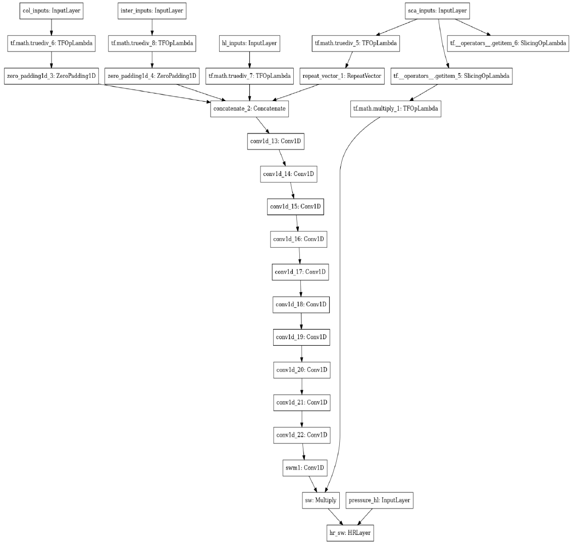
The first network we consider features a convolutional structure. Before this can be applied, the input shapes need to be standardised. Surface variables are repeated 138 times to match the 138 half-levels. Full-level fields are zero-padded at the top of the atmosphere by 1 to match 138. Interface fields are zero-padded at both the top & bottom to match 138. All inputs are concatenated along the channel dimension, resulting in 47 input channels. The learnt component of this model consists of convolutional layers, each with 64 filters, a kernel width of 5 and the Swish nonlinearity (Ramachandran, 2017). First, we use 5 convolutional layers featuring dilated convolutions (Chen et al.,2017), with dilation factors [1,2,4,8,16]. These are used to propagate information throughout the vertical column. Following these we use 5 more convolutional layers without dilation. The next step is to include a final convolutional layer with 2 channels, representing the downwards and upwards fluxes, with a sigmoid activation. This output is multiplied by two scalars, the global incoming solar radiation and the cosine solar zenith angle. This scales the output in proportion to the local incoming flux and provides our output fluxes. Finally, we use a custom layer to enact the heating rate equation outlined in 3.3.1. This takes the fluxes and half-level pressure as inputs. The graph of this model is depicted below.

We train the model for 50 epochs with a batch size of 512 and an initial learning rate of 2x10⁻⁴. The learning rate is multiplied by a factor of 0.25 after 4 epochs without validation loss improvement, with a minimal learning rate of 10-6. Our loss function is a combination of the mean-absolution-error (MAE) of the normalised flux profiles and the MAE of the heating rate. The normalised flux profile is calculated by dividing the flux profile by the incoming downwards flux. This standardises each column to be 1 for downwards flux at the top of the atmosphere and means that atmospheric columns with acute solar zenith angles, i.e. dusk/dawn are weighted equally with midday profiles. To combine the normalised MAE of the flux profile and the MAE of the heating rate we multiply the latter by 0.1, empirically finding that this led to a good balance of priorities. We select the best model on the validation dataset as the optimal model.

The second design follows that of Ukkonen (2021), who aimed to predict a similar process but for a shallower atmosphere. The design is motivated by the algorithm used in the conventional solver, which integrates down the atmospheric column, calculates interactions with the surface, integrates back up the column, and finally back down the column one final time. To mimic this, the design of Ukkonen uses a series of recurrent neural networks for each of these passes. Specifically, the network begins with a Gated Recurrent Unit (GRU, Cho et al.,2014.), which integrates from the top of the atmosphere to the surface, i.e. 137 steps of the GRU, where the appropriate full-layer variables are inputted at each step down the atmosphere. The output of the GRU at the surface is combined with the surface albedo, before applying a Dense layer to the output to mimic the reflectance at the surface. A second GRU is then integrated from the surface to the top of the atmosphere, where the layerwise inputs are the inputs and outputs from the previous GRU layer. A third GRU integrates back down the column, with the inputs and outputs from both prior GRU layers. Each of the GRU layers use 64 units, tanh activation and sigmoid recurrent activation. Finally, we reproduce the last features of the convolutional model outlined in experiment 1; a convolutional layer with 2 channels, multiplication by incoming flux and a heating rate layer. This model, without these final steps, is depicted in Figure 4 of Ukkonen (2021), and a representation of the graph is shown in Figure 5. In total, the model has 85,698 trainable parameters. Training follows that of the convolutional model, except the initial learning rate is set to 0.001.

The third experiment is an extension of the convolutional model in experiment 1. The only changes introduced are two self-attention layers (Vaswani 2017), which are introduced after the dilated convolution and before the final convolution layer. These self-attention layers have 8 heads and a key dimension of size 8. The purpose of introducing the self-attention layers is to aid the propagation of information throughout the vertical column. As these layers enable rapid exchange of data in the vertical dimension we remove the dilation from the early convolution layers. In total, the model has 233,922 trainable parameters. The graph of the network is depicted below.

During testing, we found that the default behaviour on NVIDIA A100s with Tensorflow to use Tensor Float 32 led to worse scores. Therefore this behaviour was removed for the training of this model, resulting in single precision being used for all calculations.

The graphs below show the training and validation curves for the three experiments, with the left plot showing the results for the fluxes and the right plot the heating rates. For the fluxes, experiment 3 produces the best results on both the training and validation dataset. For the heating rates, the RNN from experiment 2 produces the best results, but only by a small margin.

The below figure plots four example columns from the test data for the shortwave fluxes (down & up) and the heating rate. The x-axis corresponds to the vertical dimension, with model level 1 corresponding to the top of the atmosphere. The RNN from experiment 2 is depicted as the prediction. Overall, extremely good agreement is seen, with only a small degradation in the upwards flux at the top of the atmosphere for example 1.

On the test data the same picture is observed, the results are displayed in the table below. Both experiments 2 & 3 can be considered optimal depending on the importance of the two components.

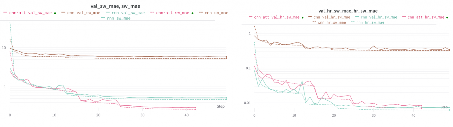
Experiment #	Loss	SW MSE	SW MAE	SW HR MSE	SW HR MAE
1	0.0299	1627	12.2600	0.0963	0.0763
2	0.0017	1.6180	0.4290	0.0004	0.0061
3	0.0014	0.5000	0.2498	0.0005	0.0070

The final test of any model for this application is coupling it into the IFS atmospheric model to assess forecast quality. This step will be carried out next to differentiate between the two models. The relative inference costs will also be an important factor if the scientific quality of the forecasts are comparable for both models. A method for introducing these models into the Fortran codebase has been developed4. but this has not yet been tested using GPUs for the inference.

Further model optimisation is surely possible, as some of the hyperparameters in the above models have not been fully explored.

These and other architectures will be examined for the longwave aspect of the heating problem.

Finally, the models for this application will have further value, providing differentiable models for data assimilation. Over the next year we will establish the best methodology for generating the tangent linear versions of our models, and then testing their stability within data assimilation.