Improved local weather predictions in forecast post-processing

 https://gitlab.jsc.fz-juelich.de/esde/machine-learning/downscaling_maelstrom/-/tree/develop
The code can be accessed in our project repository. The corresponding experiments can be run from the branch in Table 9. The code can be downloaded via a CliMetLab plugin.
Branch name for experiment 1, 2:

michael_issue#039_maelstrom_deliverable1.3

Branch name for experiment 3:

bing_issue#41_embedding_date_and_time

Branch name for experiment 4, 5:

bing_issue#031_swinIR

This application is being delivered by Forschungszentrum Jülich.

This app explores the application of deep neural networks for statistical downscaling of meteorological fields. Inspired by the success of super-resolution techniques on images in the computer vision domain, different model architectures will be explored for downscaling the 2m temperature over complex terrain. These architectures, along with the deployed dataset, are described subsequently.

A dataset for a pure downscaling task has been published. Pure downscaling in this context means that the deep neural network is only learning a mapping from the coarse-grained input data to the high-resolved target data. Systematic biases due to the truncated spatial resolution of the input data are not part of the downscaling task, even though their reduction constitutes one of the central aims when increasing the spatial resolution of atmospheric models (see, e.g., Giorgi and Gutowski et al., 2015).

In this deliverable, we aim to extend the statistical downscaling task by creating a dataset that allows to incorporate both, increasing the spatial resolution of coarse-grained meteorological fields to highresolved field including bias correction. For this, we choose the ERA5-reanalysis as the input and the COSMO-REA6 reanalysis as the target dataset.

The ERA5-dataset constitutes a global reanalysis product which is based on ECMWF’s Integrated Forecasting System (IFS) model, version CY41R2 (Hersbach et al., 2021). Data is available from 1959 until near real-time so that the spatio-temporal coverage is comprehensive. However, the underlying model runs on a reduced Gaussian grid with a spacing of about 31 km (Δx_ERA5 ≃ 0.2825°) which is fairly coarse-grained.

By contrast, the COSMO-REA6 dataset is provided on a rotated pole grid with a spacing of about 6 km (Δx_CREA6,rot = 0.055°, see Bollmann et al., 2015 a,b). Thus, the spatial resolution is about five times higher than the (global) ERA5-reanalysis product. Anyway, the COSMO-REA6 is limited to a domain covering Europe (880x856 grid points) and the reanalysis data is only available between 1995 and August 2019. The COSMO model (version 4.25) developed at the German Weather Service (DWD) was used to create the regional reanalysis dataset.

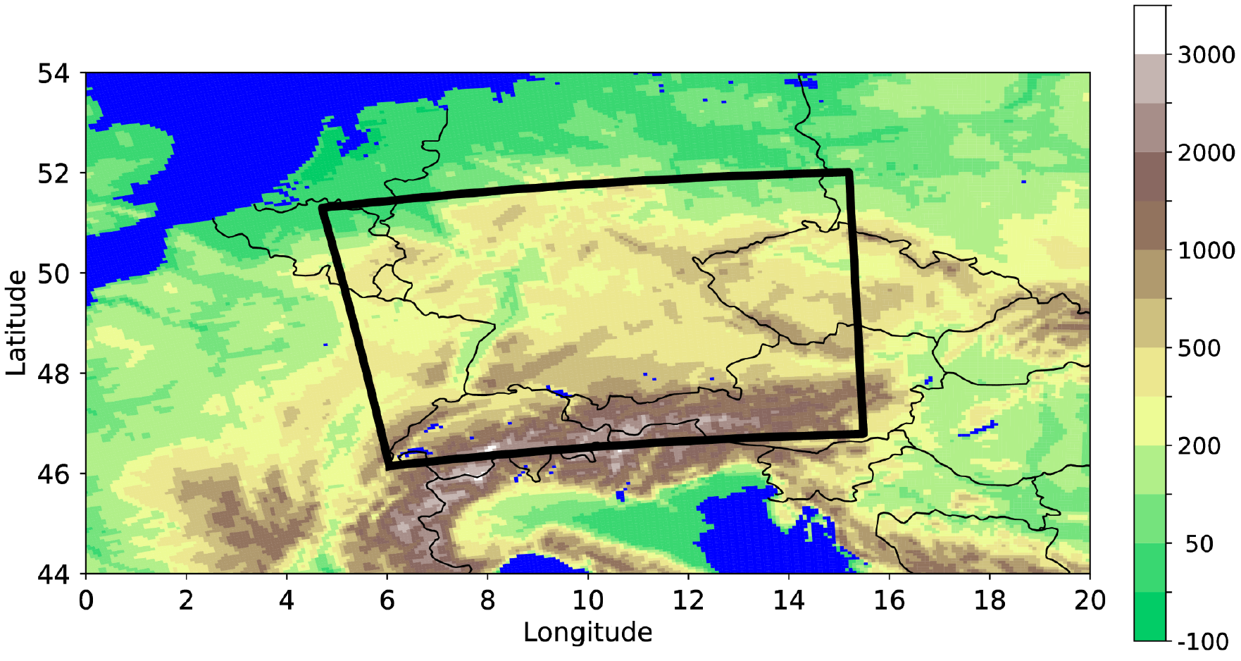
For the Tier-2 dataset of this deliverable, we harmonise data from 2006 to 2018 over a target domain with 120x96 grid points covering large parts of Central Europe. Although the target domain is just a subset of the COSMO-REA6 domain, it constitutes a suitable region for the downscaling task due to the underlying complex topography of the German low-mountain range and parts of the Alps (see figure bwlow). To avoid mismatches in the underlying grid projection of both datasets, the ERA5-reanalysis data is remapped onto a rotated pole grid with Δx_ERA5,rot = 0.275°. The same remapping procedure as described in deliverable 1.1 is deployed.

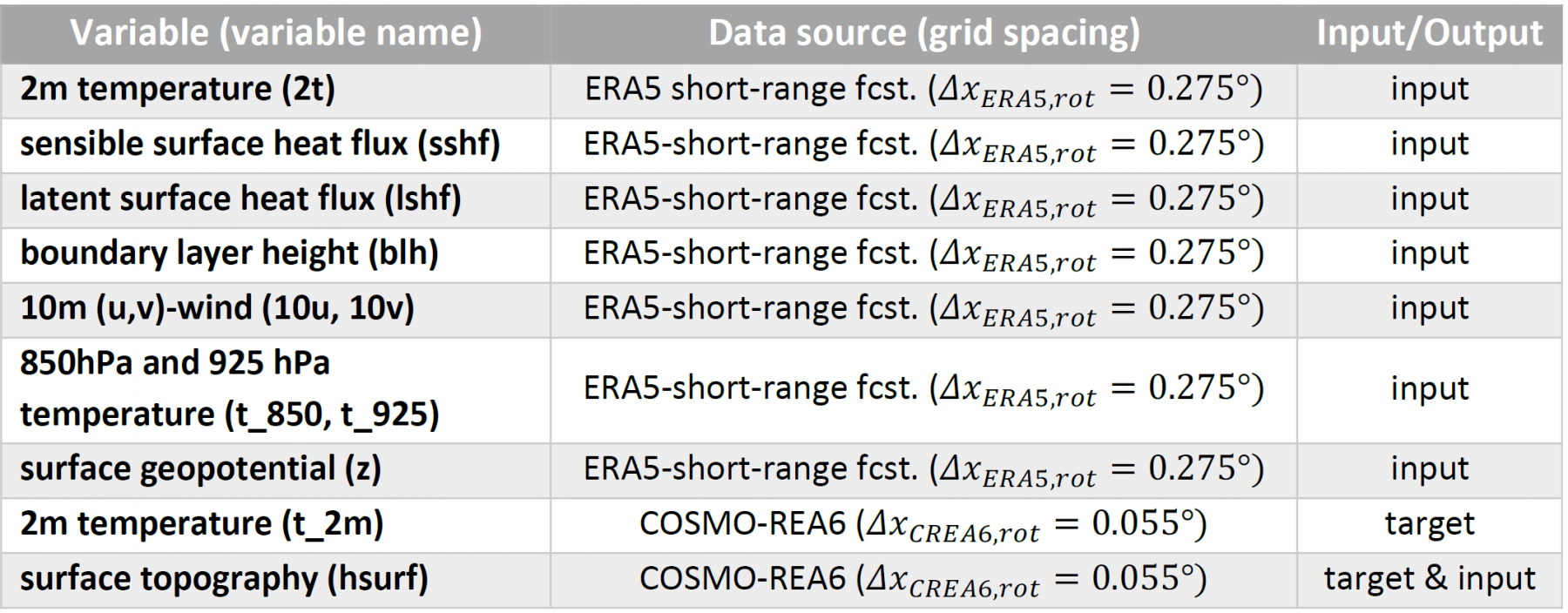
For the particular task of downscaling the 2m temperature (T2m), several predictor variables are chosen from the ERA5-dataset to encode the state of the planetary boundary layer in a data-driven way. This constitutes a notable difference to the Tier-1 dataset which only inputted the surface topography in addition to the coarse-grained T2m-field. By extending the set of predictor variables, the neural network is supposed to be applicable to arbitrary daytimes and seasons, whereas the neural network application with the Tier-1 dataset is limited to daytimes at noon of the summer half year. An overview of the predictor variables from the ERA5-dataset is provided in Table 8. Note that the usage of surface heat fluxes is only possible with the ERA5 short range forecasts that are initiated at 06 and 18 UTC, respectively, from the analysis fields within the 12-hour assimilation window (Hersbach et al., 2021). To reduce the footprint of spin-up effects, data between forecast hour six and 17 are used to construct the input data.

Similar to the Tier-1 dataset, the 2m temperature from the COSMO-REA6 dataset is complemented by the surface topography of the target domain. According to Sha et al., 2020, adding this static field to the predictands encourages the neural network to be orography-aware.

In total, the final dataset then comprises 111.548 samples of which data from 2017 and 2018 are used for the validation and testing (8748 samples each), respectively, while the remaining 11 years of data are reserved for training (94,052 samples). Note that this data split-approach maximises the statistical independence between the datasets in light of the autocorrelation of atmospheric data as argued in Schultz et al., 2021. The datasets are stored in netCDF-format and reside in about 45 GB of memory for the training data and 4.2 GB for the validation and the test dataset, respectively.

For downscaling the coarse-grained ERA5-data to the high-resolved 2m temperature field of COSMOREA6, we test the two neural network architectures, U-Net and WGAN.

U-Net

A U-Net architecture is used as the baseline model for 2m temperature downscaling. The original U-Net was first proposed by Ronneberger et al., 2015, and used for biomedical image segmentation. This architecture deploys convolutional layers as building blocks and is capable of extracting features at various spatial scales using symmetrical encoder-decoder blocks. The U-Net architecture used in this study is adapted from Sha et al., 2020, and comprises three upand down-sampling blocks for the encoder and decoder, respectively. Each down-sampling block consists of a convolutional layer followed by max-pooling to reduce the number of grid points in the horizontal plane. Skip connections connect the encoder with the decoder which applies deconvolutional layers to reverse the spatial data reduction of the encoder. A visualisation of the U-Net including some further information on the configuration is provided in the figure below (the U-Net constitutes the generator in WGAN).

WGAN

While the U-Net architecture turns out to perform reasonably well on the Tier-1 dataset in terms of the RMSE, the spatial variability of the downscaled 2m temperature field is underestimated. This is a well-known issue of pure convolutional network architectures since they are prone to produce blurry images in computer vision applications (see, e.g., Bulat et al., 2018).

To address this issue for the downscaling application on the Tier-2 dataset, we integrate the U-Net as a generator into a Generative Adversarial Network (GAN). In computer vision, GANs have become state-of-the art for super-resolution tasks since the study of Ledig et al., 2017. By incorporating a discriminator to distinguish between real and generated data in an adversarial optimization process, the generator is trained to fool the discriminator. By doing so, the generator is encouraged to produce (super-resolved) data that share the same statistical properties as real data which, in turn, implies that small-scale features have to be generated (Goodfellow, 2020).

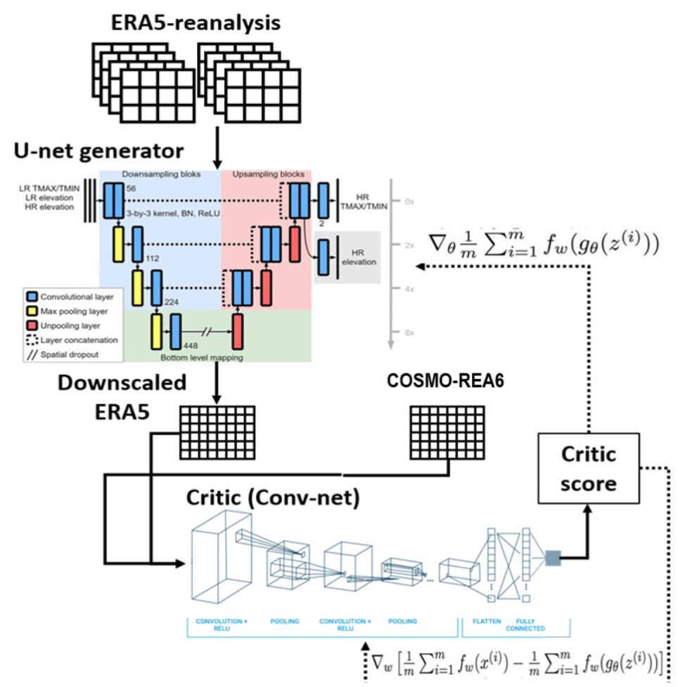
Despite this appealing property, GANs are often hard to train since a balance between the generator and the discriminator must be retained throughout the training. To stabilise the optimization process, Wasserstein GANs (WGANs) have been proposed where the discriminator is replaced by a critic (Arjovsky et al., 2017). Deploying a critic instead of a discriminator is beneficial since the critic does not saturate and thus is capable of providing clean gradients during training. By contrast, discriminators may suffer from vanishing gradients for which optimization gets stuck. While the aforementioned U-Net is deployed as the generator, a neural network comprising four convolutional layers, a global average pooling layer and a final dense layer is set-up as the critic for our downscaling task. The complete WGAN architecture is illustrated in Figure 10. In total, the WGAN model comprises about 5 million trainable parameters of which 1.5 million (3.5 million) are part of the critic (generator).

Three different experiments were conducted with the two presented neural network architectures: For Experiment 1 and 2, the Tier-2 dataset is fed to the U-Net and to the WGAN. The main focus of these experiments will be to check if the adversarial network architecture is capable of increasing the spatial variability of the downscaled 2m temperature field.

For Experiment 3, the training on WGAN is repeated with additional datetime embeddings for the input. The motivation for embedding the month of the year as well as the hour of the day is to ease encoding of the planetary boundary layer state in the neural network which is known to be a main driver of 2m temperature variability (see, e.g., Akylas et al., 2007).

For all experiments, the U-Net is trained for 30 epochs while the generator of WGAN is trained for 40 epochs. The initial learning rate of the U-Net model is set to 1 ∗ 10-4 which is then subject to exponential learning rate decay after five epochs (the decay exponent is set to -0.1). For the WGAN, different initial learning rates are set for the generator and the critic. However, both learning rates are decayed between epoch five and ten. The respective learning rates schedules have been obtained empirically from tuning.

The loss function of the U-Net constitutes the Mean Absolute Error, also known as L1-error, of the (normalised) 2m temperature. For the WGAN, the same reconstruction loss is weighted by a factor of 1000 and combined with the Wasserstein distance between the generated and real data. Furthermore, a gradient penalty (weighted by 10) is deployed for the WGAN to fulfil the 1-Lipschitz constraint.

In the following, we briefly evaluate the experiments in terms of the RMSE, the bias and the spatial variability. For the latter, the domain-averaged amplitude of the horizontal gradient from the downscaled 2m temperature field is compared against the ground truth data. When the gradient amplitude ratio equals 1, the local variability of both 2m temperature fields is the same, whereas it is underestimated (overestimated) for ratios smaller (larger) than 1.

Experiment 1 & 2

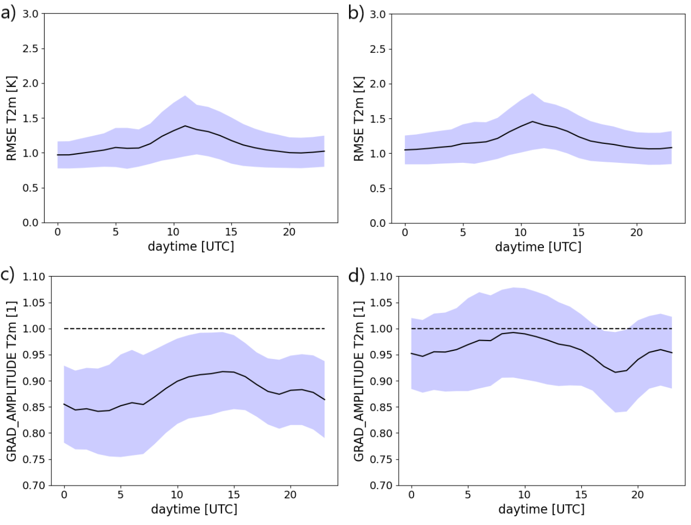
The first row of the figures above shows the RMSE obtained with the U-Net (a) and with the WGAN (b) as a function of daytime for the testing data from 2018. The performance of both models is comparable, even though the U-Net attains marginally smaller RMSE-values. It is seen that the error tends to be larger at around local noon when the RMSE approaches 1.5 K, whereas it is smallest overnight. Inspecting the bias shows that both neural networks attain a value close to 0 (not shown). Slightly larger systematic deviations are just present after midnight (cold bias) and in the morning hours (warm bias).

However, in terms of the spatial variability, the WGAN significantly outperforms the U-Net which underestimates the amplitude of the 2m temperature gradient by more than 10% on average (second row of figure above). Especially between midnight and morning, the spatial variability is largely underestimated with the U-Net indicating that the 2m temperature field is too smooth. By contrast, WGAN nearly manages to recover the spatial variability of the ground truth data at early noon and only slightly underestimates it for other daytimes (except from a short period in the evening hours). Thus, the integration of the U-Net model as a generator to the WGAN turns out to be beneficial since the spatial variability gets substantially more realistic, while point-wise error metrics remain largely unaffected.

However, closer inspection of the results reveals persisting issues for the WGAN.

The figures above presents the diurnal cycle of the gradient amplitude ratio during summer, while Figure 12 (b) shows the temporally averaged RMSE over the target domain at 12 UTC for the same season. It is seen that the WGAN clearly underestimates the spatial variability over day and that the error is largest for the Alpine region. During this time, the PBL is typically well mixed due to strong solar heating which introduces a high spatial variability over complex terrain due to adiabatic or super-adiabatic near surface lapse rate. Obviously, the U-Net has problems to properly encode this PBL state from the input data, so that the spatial variability due to the underlying terrain is notoriously underestimated which also introduces systematic biases (not shown). In the following experiments, we therefore probe if additional daytime and season embedding (hour of the day and month of the year) can support proper encoding which in turn would improve the results for the summer season.

Experiment 3

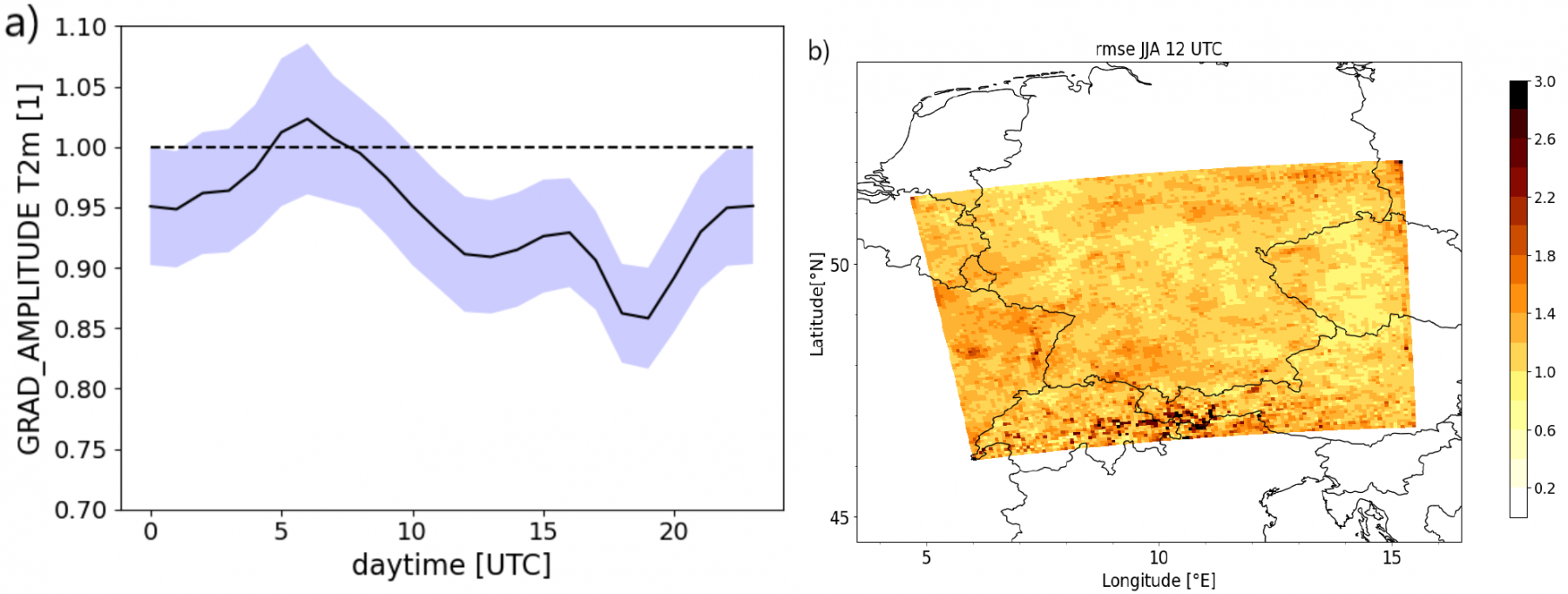
To embed the daytime and the season (date embedding), two additional input layers are added to the generator of the WGAN architecture. The hour of the day as well as the month of year corresponding to each sample are converted to one-hot vectors (of shape 24 and 12, respectively) which are then projected to a scalar value via a trainable, fully connected layer. By doing so, a data-driven encoding of the date-information can be learned by the neural network via backpropagation. Finally, the scalar value is expanded to a 2D-tensor to allow concatenation along the channel-dimension of the gridded ERA5-input data.

In general, the added value of the date embedding is fairly small. In terms of the RMSE and the gradient amplitude ratio of T2m, only small improvements can be diagnosed. While the small improvements are consistently observed for most daytimes and seasons (cf. Figure 13), the above mentioned issues around noon during the summer months persist:

The RMSE still tracks quite high during this time, although we note a more pronounced improvement of spatial variability (see figure below). All in all, further investigation is required to come up with a more robust added value of the datetime embedding.

In the future, further effort to improve the performance of the downscaling models will be pursued. The main step comprises the following action items:

• The downscaling dataset will be completed by extending the training data back to 1995. Note that the current Tier-2 dataset is restricted to the period 2006-2018. The extension of the dataset will also require efficient data streaming from the netCDF-files. Currently, all the data are loaded into a memory which limits the application of the current source-code to HPC-systems equipped with large RAM. In the future, a more flexible input data pipe will be developed to relax the memory restrictions of the current approach.
• A systematic analysis on the added value of the predictor variables will be conducted. Additional input parameters such as the total cloud cover or predictor variables from previous time steps will be considered to improve the data-driven encoding of the PBL state which in turn is expected to improve the downscaling product.
• Further hyperparameter tuning for the deployed U-Net and WGAN will be undertaken. Other neural network architectures such as the downscaling network suggested by Leinonen et al., 2020, or Stengel et al., 2020, will also be considered as competing models.

In addition to improving the neural networks for downscaling the 2m temperature, we plan to extend the application of the ERA5 to COSMO-REA6 downscaling task to other meteorological fields. Specifically, downscaling of the incoming solar radiation or the wind at 10m above ground, which are both relevant for the renewable energy sector, will be tested as well. The overarching target is to provide a comprehensive benchmark dataset for downscaling that can be applied to different downscaling tasks. We note that an increased demand for such a benchmark dataset has recently arisen in the meteorological domain as, for instance, discussed in the Machine Learning for Climate Science-session of the EGU General Assembly 2022.

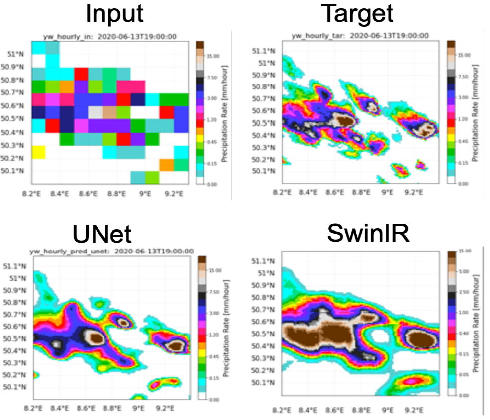
Finally, we also aim to extend our application to the challenging task of downscaling precipitation forecasts. In particular, we aim to make use of precipitation forecasts from the IFS HRES which constitutes the world-leading global NWP model operational at ECMWF. The IFS HRES forecasts are provided on a grid with Δx_IFS ≃ 9 km which is still too coarse to represent the high spatial variability of convective precipitation. Thus, rain-gauge adjusted radar observations provided by the RADKLIM dataset with Δx_RADKLIM = 1 km (Winterrath et al., 2017) will be used as the target of the downscaling task which will furthermore be extended to a probabilistic framework to account for the chaotic nature of precipitation processes. For this purpose, recent model architectures based on vision transformers such as the SwinR network will be tested and developed (Liang et al., 2021). One advantage of transformer-based models is that they can retain an optimised computational costaccuracy trade-off. Our first results demonstrate that the training time of the SwinIR-downscaling model is much faster than the U-Net architecture. Preliminary results from a (deterministic) SwinIRdownscaling model together with the downscaled product from a U-Net model are provided in Figure 15. It is seen that the downscaled precipitation field is still too coarse for both models and that artefacts due to the shifting window-approach in SwinIR reside in the downscaled product (Zhang et al., 2022). Thus, further development of the model architectures is required to improve the performance of the models, so that they can be compared to recent downscaling advances described in the study by Price and Rasp, 2022, and Harris et al., 2022.