Improved ensemble predictions in forecast post-processing

 https://github.com/spcl/ens10
Data may be accessed via a CliMetLab plugin, installed as:

pip install climetlab climetlab-maelstrom-ens10

The ENS-10 dataset can then be downloaded using

import climetlab as cml
cml.load_dataset('maelstrom-ens10')

Full details on experiments and additional examples can be found at github.             

This application is being delivered by ETH's Scalable Parallel Computing Lab.

Weather prediction needs to not only forecast the most likely future scenario, but also provide a probability distribution over specific weather events. Traditionally, existing numerical weather prediction systems achieve this by generating many ensemble members, or perturbed realisations of a weather simulation, which are then used to estimate probability distributions for key quantities, such as precipitation. However, achieving high-quality distributions requires many ensemble members, which is computationally expensive.

To address this challenge, Application 4 utilises deep neural networks to post-process these ensemble members to improve the quality of the probability distribution. As a first step, we have developed a new dataset, ENS-10, and an associated set of ML models, to serve as a benchmark for the ensemble post-processing task. This dataset is also documented in Ashkboos et al., 2022, which provides additional details.

The ENS-10 dataset consists of ten perturbed ensemble members spanning twenty years (1998–2017) for medium-range weather forecasts (lead time 48 hours). This data was introduced in MAELSTROM Deliverable 1.1, and we summarize key details here. Each ensemble member contains a selected set of key weather variables over eleven pressure levels (10, 50, 100, 200, 300, 400, 500, 700, 850, 925, and 1000 hPa):

• U wind component,
• V wind component,
• Geopotential,
• Temperature,
• Specific humidity,
• Vertical velocity,
• and Divergence.

The dataset also contains important surface variables:

• Sea surface temperature,
• Total column water,
• Total column water vapour,
• Convective precipitation,
• Mean sea level pressure,
• Total cloud cover,
• 10 m U wind component,
• 10 m V wind component,
• 2 m temperature,
• Total precipitation,
• and Skin temperature at the surface.

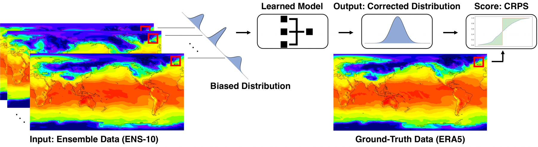
ENS-10 is generated from reforecasts run at ECMWF, with two forecasts per week. The data are provided on a structured grid at 0.5° resolution.

As part of ENS-10, we define the prediction correction task, where the goal is to correct the output distribution of a set of ensemble weather forecasts. Formally, given a set of ensemble members at time T and lead time L, the task is to predict a corrected cumulative distribution function (CDF) for a variable of interest (e.g., temperature) at time T + L. In ENS-10, we consider three variables for this task: 2 m temperature (T2m), temperature at 850 hPa (T850), and geopotential at 500 hPa (Z500). Years 1998–2015 are used as training data, and years 2016–2017 are used as a test set. The ERA-5 reanalysis dataset produced by ECMWF is used to provide ground-truth values.

A potential solution is evaluated with two different metrics. The first is the standard continuousranked probability score (CRPS) (Zamo et al., 2018). CRPS generalises the mean absolute error for the case where forecasts are probabilistic. In addition, in Ashkboos et al., 2022, we introduce the Extreme Event Weighted CRPS (EECRPS) metric to evaluate a solution specifically for extreme events, which are of particular interest in probabilistic forecasting. EECRPS is the pointwise CRPS weighted by the Extreme Forecast Index (EFI), which measures the deviation of the ensemble forecast relative to a probabilistic climate model.

We provide three baseline ML methods: Ensemble Model Output Statistics, a multi-layer perceptron, and a U-Net.

Ensemble Model Output Statistics (EMOS) (Gneiting et al., 2005) is a statistical method based on a linear relation between the ensemble values and the corrected mean and variance. It computes the mean and standard deviation of the corrected distribution by fitting a linear function to the ensemble members.

A multi-layer perceptron (MLP) is a set of full-connected layers, each followed by a non-linearity (e.g., ReLU). We apply an MLP with one hidden layer to ENS-10, which estimates the pointwise corrected mean and standard deviation of the output distribution. The network has 25 and 17 input dimensions for the volumetric and surface variables, respectively (two inputs for each variable in the dataset and three for XYZ coordinates). The hidden layer has dimension 128 and uses a ReLU activation.

The MLP model operates on each grid point separately. We also apply a U-Net model (Ronneberger et al., 2015), which is widely used in image segmentation and has previously been used for ensemble post-processing (Grönquist et al., 2021).

Our U-Net baseline consists of three levels, each with a set of [convolution, batch normalisation, ReLU] modules and operates on the whole grid with 22 and 14 input dimensions for the surface and volumetric variables, respectively (two inputs for each variable). We use convolutions with 32, 64, and 128 output channels in the network’s first, second, and third levels, respectively.

We evaluate our benchmark models on the ENS-10 dataset through verification metrics CRPS and EECRPS, and additionally provide the raw ensemble’s mean and standard deviation with no correction (“Raw” in the results). Data were normalised for input. The U-Net was trained using a batch size of eight samples, while the EMOS and MLP models used one sample per batch (larger batch sizes degraded accuracy). All models were trained for ten epochs on a single A100 GPU, which took 0.75, 0.25, and 1 hours for the EMOS, MLP, and U-Net, respectively.

The table, global mean CRPS and EECRPS on ENS-10 test set for our baseline models, shows the final results of our models, trained using either ten (10-ENS) or five (5-ENS) models. We report the mean and standard deviation over three experiments for all results (except Raw, where this is not applicable).

Metric	Model	Z500 [m2s-2]		T850 [K]		T2m [K]
		5-ENS	10-ENS	5-ENS	10-ENS	5-ENS	10-ENS
CRPS	Raw	81.030	78.240	0.748	0.719	0.758	0.733
	EMOS	79.080 ±0.739	81.740 ±6.131	0.725 ±0.002	0.756 ±0.052	0.718 ±0.003	0.749 ±0.054
	MLP	75.840 ±0.016	74.630 ±0.029	0.701 ±2e-4	0.684 ±4e-4	0.684 ±6e-4	0.672 ±5e-4
	U-Net	76.660 ±0.470	76.250 ±0.106	0.687 ±0.003	0.669 ±0.009	0.659 ±0.005	0.644 ±0.006
EECRPS	Raw	29.80	28.78	0.256	0.246	0.258	0.250
	EMOS	29.100 ±0.187	30.130 ±2.166	0.248 ±3e-4	0.259 ±0.018	0.245 ±0.001	0.255 ±0.018
	MLP	27.860 ±0.006	27.410 ±0.010	0.240 ±1e-4	0.234 ±2e-4	0.233 ±2e-4	0.229 ±2e-4
	U-Net	27.980 ±0.240	27.610 ±0.490	0.235 ±0.003	0.230 ±0.002	0.223 ±5e-4	0.219 ±0.001