
Empowering weather and climate forecast
climetlab-maelstrom-power-production plugin
notebooks/pca.ipynb

Forecasts for power production of renewable energy resources are prone to uncertainty. While forecasts for power production from solar resources usually exhibit low errors (< 10%) that are quite stable in time, wind power forecasts typically suffer from larger uncertainties (≳ 10%) that have a higher variance.
To produce power production forecasts for individual plants and sites, the developed ML models consider small-scale, local weather conditions. The past has shown, though, that the forecast uncertainty may well be affected by large-scale weather patterns with time scales exceeding the maximum forecasting leadtime. As a consequence, we aim to investigate whether models informed by large-scale weather regimes (LSWRs) over Europe have the ability to reduce the uncertainty of power forecasting for wind and solar resources.
Here, we use an entirely data-driven approach to classify LSWRs. The data consist of a time series with multiple physical quantities that describe the weather conditions on multiple pressure levels on a large grid covering the whole of Europe. Hence, the dataset is high-dimensional. To apply a classification of weather patterns in the data, we perform a dimensionality reduction of the multi-level grid time series and apply a classification on the resulting low-dimensional projection of the data.
In the first approach, we want to study each individual LSWR found in the data and get information about their characteristics including stability and endurance. Here, we want to compare the different classes of LSWRs to the so-called Großwetterlagen (GWL) defined by the German Meteorological Service (Deutscher Wetterdienst, DWD). The DWD created a catalogue of 40 GWL characterised by geopotential, temperature, relative humidity, and zonal and meridional wind component on multiple pressure levels. GWL has certain characteristics and are stable up to several days, and hence allow to generalise the evolution of small-scale weather conditions during the appearance of the respective GWL.
We then want to investigate how power production forecast uncertainty behaves for the different LSWRs since we suspect that there is a relation between LSWR classes and the prediction errors. Using this information, we aim to develop more advanced models that have knowledge about present LSWRs (LSWR-informed models), and thus, are more robust against changes in small-scale weather conditions.
The underlying data are from the ECMWF IFS HRES model. A detailed description can be found in the document of the Deliverable D1.1 in Section 3.6.11 The data cover a time range of 2017-2020 with an hourly temporal resolution resampled to a daily resolution where we calculate the daily mean of each physical quantity. The grid covers the whole of Europe with an area of 35°N to 70°N and 25°W to 30°E and a spatial resolution of 0.1°N and 0.1°E. Each physical quantity is given on a set of multiple pressure levels (500hPa, 800hPa, 925hPa, 950hPa and 1000hPa). Since we aim to compare the LSWRs that we find in the data to the GWL defined by DWD, we similarly use the following physical quantities at the 500 hPa pressure level:
The classification of LSWRs is done by applying a clustering algorithm on the data that assigns each individual time step to a cluster, where outliers are allowed. Each cluster thus represents a unique LSWR that occured over the time span of the time series. Outliers here represent transition phases between different states of the system.
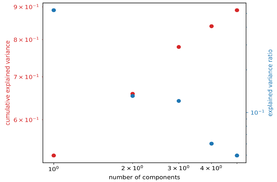
To allow classification of the high-dimensional time series grid data, we apply a dimensionality reduction algorithm (Principal Component Analysis, PCA). PCA finds a set of orthonormal vectors (principal components, PCs), where each of which accounts for a certain amount of variance of the dataset (if the data were projected onto that vector). Here, the fraction of the variance represented by each PC is in ascending order. I.e., the first component accounts for most of the variance in the dataset, the second for the second most, and so forth.
However, we only use a subset NPCs of the retrieved PCs to transform the original data into the lowdimensional PC space. The PC space is a multi-dimensional vector space that represents the phase space of the dynamical system described by the data. To avoid the curse of dimensions, we use only a reduced amount of PCs for the transformation such that the PCs reflect most of the variance of the data.
For clustering the states of the dynamical system in PC space, we use the Hierarchical Density-Based Spatial Clustering Algorithm for Applications with Noise (HDBSCAN) by Malzer and Baum (2019), which is a modification of the DBSCAN algorithm (Ester et al., 1996). As implied by the name, the algorithm finds high-density regions in a given data set that represent clusters of related data points. Data points outside of such high-density regions (outliers) are classified as noise.
The PCA is performed on the whole dataset. To allow a PCA on a time series grid, the data have to be flattened by concatenating the rows (representing the different latitudes) of the grid for each physical quantity. The flattened grids of all investigated physical quantities are then concatenated as well.
However, we use only NPCs = 3 to transform the data into PC space. This is because we only have 10³ data samples (4 years of data with roughly 365 days each). Choosing more PCs would require more data (curse of dimensions). I.e., using N PCs would require at least 10
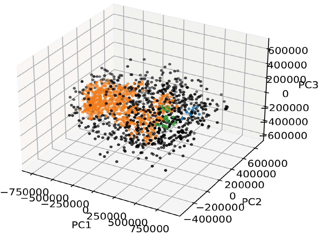
Before applying the clustering, the data are transformed into the 3-D subspace of the PC space. The result reflects the phase space containing all states of the dynamical system throughout the given time span (2017-2020).
Within this space, we perform a clustering to find recurring states where the system frequently resides in. Each retrieved cluster then represents a unique LSWR, i.e. all clusters represent the ensemble of LSWRs that our system resided in during the given time range. Each data point in a cluster hence reflects the time steps within the time series where the LSWR of the respective cluster appeared. This allows a thorough statistical analysis of each LSWR.
The clusters (LSWRs) are then statistically analysed such that we retrieve information about the LSWRs in general (total abundance, mean and standard deviation of their duration). In addition, we plan to visualise the appearance of individual LSWR clusters at all time steps.
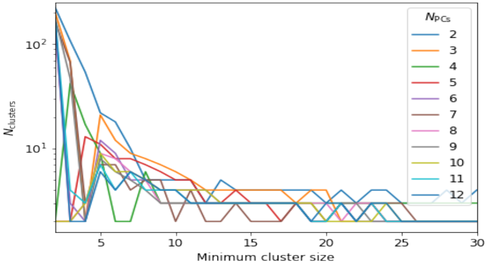
After transforming the data into the 3-dimensional PC space, applying the HDBSCAN yields Nclusters = 3 clusters, where ~ 60% of the data points (days) are classified as outliers (see figure below). Here, we use min_cluster_size=10. A hyperparameter study where we varied the number of PCs used for dimensionality reduction from 2–12 and the minimum cluster size from 2–30 has shown that the number of clusters found by the algorithm converges at a minimum cluster size of ~ 10 (see figure below).
The clusters represent areas in the low-dimensional phase space of our dynamical system where the system repeatedly resided in, i.e. the LSWRs we are actually interested in.
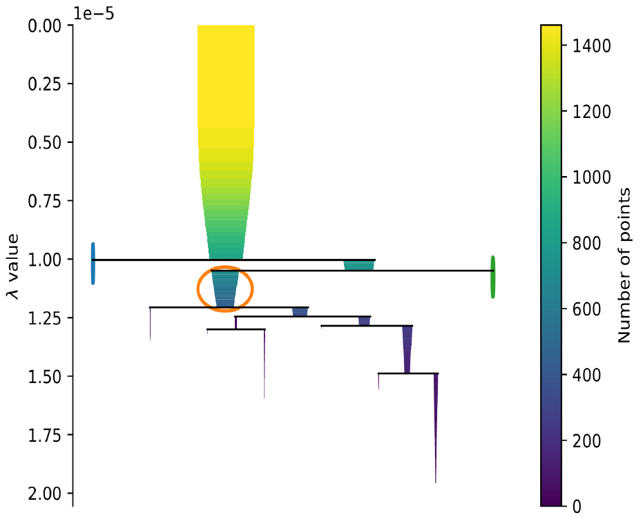
The result of the PCA and HDBSCAN is not very promising since we only find three clusters, which is not granular enough for our purpose. The three clusters may in fact represent larger weather circulation patterns. However, our aim is to find more clearly separable LSWRs with durations in the order of days. Moreover, the amount of data points identified as noise (~60%) is too large and drastically reduces the number of potential days that can be used for investigating any relationship of LSWRs to renewable power production.
Our next step will be to apply Dynamic Mode Decomposition (DMD) for dimensionality reduction and compare its results to that of the PCA. DMD is especially suited to find dominant modes in dynamical systems, originally developed for and applied to fluid mechanics by Schmid and Sesterhenn (2008). An advantage of DMD is that it is an entirely data-driven approach to analyse dynamical systems without requiring any information about the underlying equations of motion.