https://github.com/metno/maelstrom-train Installing the python package in the repository
provides the command-line tool maelstrom-train, which starts a run based on configuration defined
in YAML files. This includes options for the data loader, models, training, optimization, loss, and
output. The exact configuration of each experiment is documented in the settings found in etc/exp1.yml, etc/exp2.yml, and etc/exp3.yml. Use the following run commands:
The goal is to produce high resolution (1x1 km) hourly temperature forecasts 58 hours in advance for the Nordic countries.
Dataset
The dataset includes a range of predictors:
Predictor name
Unit
Has leadtime?
2m temperature control member
°C
Yes
2m temperature 10% from ensemble
°C
Yes
2m temperature 90% from ensemble
°C
Yes
Cloud area fraction
1
Yes
Precipitation amount
mm
Yes
10m x wind component
m/s
Yes
10m y wind component
m/s
Yes
2m temperature bias previous day
°C
Yes
2m temperature bias at initialization time
°C
No
True altitude
m
No
Model altitude
m
No
True land area fraction
1
No
Model land area fraction
1
No
Standard deviation of analysis at initialization time
°C
No
The MEPS modelling system changes frequently over time as model physics, data assimilation, and ensemble perturbation methods are improved. We chose the 2-year period 2020/03/01 to 2022/02/28, which represents a time period where the model configuration remained relatively constant. Some dates in the dataset are missing due to missing data in MET Norway’s archive. The dataset includes Numerical Weather Prediction (NWP) runs that were available at 03Z, 09Z, 15Z, and 21Z. Including all forecast initialization
times for every day of the two-year period would yield too large a dataset. Instead, only one of the 4
runs is included for each day, where the provided runtime alternates from day to day. Including data
from the 4 runs is important as it forces the ML solution to deliver forecasts that work for any forecast
initialization time. Data is stored in 675 netCDF files, one for each forecast run.
Experimental setup
The prediction problem is to predict three percentiles: 10%, 50%, 90%. This means the output layer in
the ML-models have 3 predictands. This application uses the quantile score as a loss function, as
described in Deliverable D1.1.
Metric
Tier 2 dataset
Data size
6.2 TB
Grid size
2321x1796
Spatial resolution
1 km
Lead times
58 (0, 1, 2, … 58)
Time period
2020/03-2022/02
Number of predictors
14
Predictor size (time, leadtime, y, x, predictor)
675 * 58 * 2321 * 1796 * 14
Target size (time, leadtime, y, x)
675 * 2321 * 1796 * 14
The models are trained using the first 50% of the dataset (2020/03/01 to 2021/02/28). Each
experiment is trained for 1 epoch, making one pass over the training data. The training reads the dates
of the NWP runs in a random order. As a single training sample is large (i.e. only 365 samples in total),
the domain was split into 63 patches each of a size of 256x256 points to increase the number of
parameter updates in an epoch. This results in a total of 22,806 training batches and parameter
updates for one epoch.
A small validation dataset was used to record the quality of the solution as the training progresses. A
29GB subset of the total dataset was used, where 24 dates were selected that samples all months of
the year and all forecast initialization times. Additionally, the validation used only a subset of the full
domain, including part of the North sea, southern Norway, and southern Sweden. The validation grid
has size of 512 x 1024, with its southwest corner at x-index 300 and y-index 550. This was done to
keep the validation dataset small enough to fit in main memory while at the same time including a
wide variety of weather situations. Validation takes 42s and is run every time 4 input files have been
processed. This results in a ~12% performance penalty, but allows the testing stage to select the model
parameters that are best.
The model parameters that had the best validation loss during the training were saved and used for
testing. The test dataset consists of the second half of the full dataset (2021/03/01 to 2022/02/28).
Each predictor was normalised by subtracting its mean and dividing by its standard deviation. The
same normalisation coefficients were used for all grid points, times, and lead times.
Benchmark models
Four benchmark models are tested. The simplest is a linear regression (LINREG) model of the 14
predictors. This is implemented as a one-layer neural network with a linear activation function
between the inputs and outputs.
The second model is a dense neural network (DNN), where five dense layers, each with five units, are
connected by a rectified linear unit (ReLu) activation function. These layers are connected to the three
outputs by linear activation functions. Weights are shared across grid points and lead times.
The third model is based on 2D convolutional neural network (CNN) layers. The basic architecture
consists of three convolutional layers, each with a 3x3 stencil. The layers have 12, 5, and 5 filters
respectively. A dense layer connects the convolutional layers and the outputs. ReLU is used as the
activation between layers, and linear activation is used before the output layer. Weights are shared
among all lead times.
The fourth model is a U-Net model (Ronneberger et al., 2015) consisting of 3 levels, with 16, 32, and
64 output channels. The model weights are shared among all lead times. The convolution size is 3x3
and the up and downsampling ratio is 2.
Additionally, the models are compared against the raw model output (RAW) that has not been postprocessed.
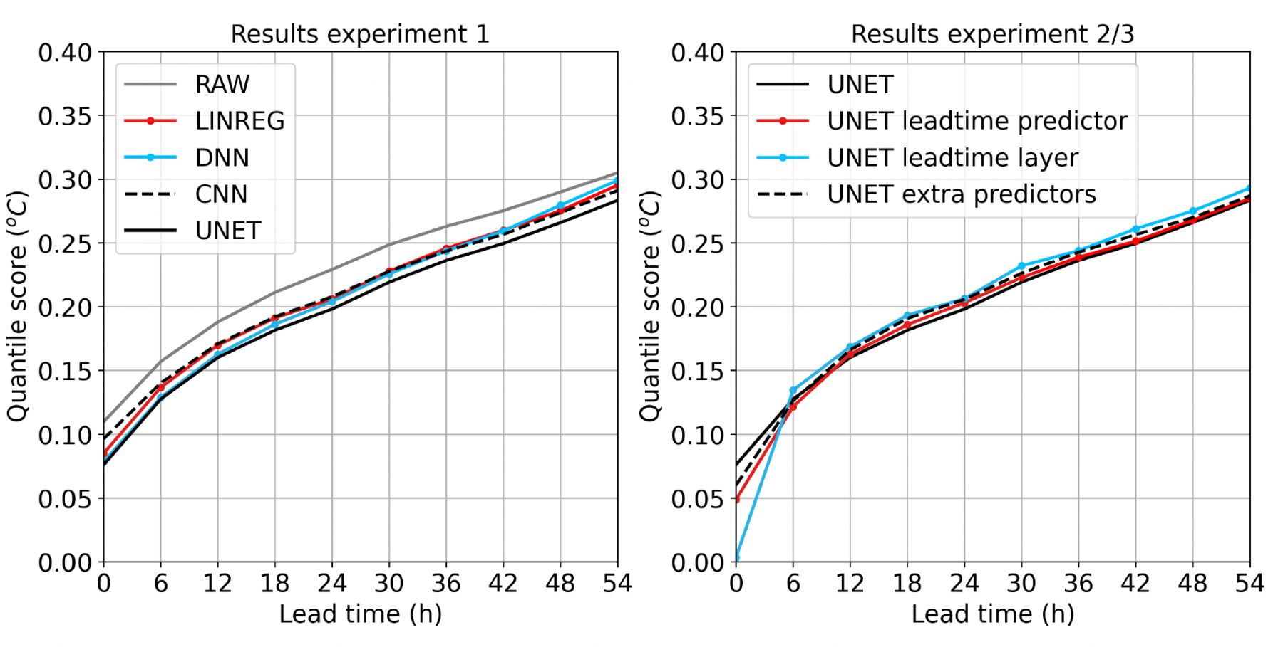
Experiment 1: Comparing benchmark models
In this experiment, we compared the performance of RAW, LINREG, DNN, CNN, and U-Net (see Figure
1 and Table 3 below). All models improve the forecast accuracy over RAW by 6-11%. CNN performed
similarly to the simpler LINREG and DNN networks, suggesting that the added complexity isn’t able to
extract complex relationships between the input and output. The more complex UNET model,
however, performed better than the other models. We did not analyse the reason for the performance
increase, but we suspect it is related to the model’s ability to detect large scale features.
Experiment 2: Comparing leadtime-dependent weights vs. leadtime as a predictor
The prediction task produces forecasts for all 59 lead times simultaneously. We know that some
predictors (e.g., bias_recent) are more relevant to early lead times than later ones. To introduce lead
time information into the models, we compare adding lead time as a (static) predictor field and adding
a locally-connected layer at the end where each lead time has different parameters. We tested this
on the best model from experiment 1 (U-Net).
Adding lead time as a predictor led to a small improvement of scores for lead times 0-6h, but no
noticeable improvement later on. The lead time layer significantly improved scores for lead time 0,
but reduced the quality for all lead times after that. The overall modest improvements from lead
time information was surprising to us, but may indicate that lead time information can be inferred
by the model (e.g. the spread of the ensemble is a proxy for lead time).
Experiment 3: Adding new features
In this experiment, new features were added to the input. These include the x and y grid values, the
month of the year, and the hour of the day. We expect these predictors will aid the model in
differentiating seasonal, diurnal, and spatially varying biases. We tested this on the model that
performed best in experiments 1 and 2 (U-Net). We did not, however, find a noticeable difference in
quality when introducing these features.
Test scores for the different experiments as a function of forecast lead time.
Model
Parameters
Test loss
Improvement
Experiment 1
RAW
0
0.2249 °C
0 %
LINREG
45
0.2094 °C
6.89 %
DNN
183
0.2067 °C
8.09%
CNN
2,437
0.2091 °C
7.03%
UNET
115,893
0.1995 °C
11.29%
Experiment 2
UNET leadtime predictor
116,040
0.1986 °C
11.69 %
UNET leadtime layer
119,895
0.2043 °C
9.16%
Experiment 3
UNET leadtime layer and extra predictors
116,628
0.2032 °C
9.65%
Outlook
We will investigate several approaches to further improve the predictive accuracy of the models and
the computational performance of the training pipeline.
Improving predictive accuracy
The experiments showed that the U-Net is a promising model capable of beating simpler models. We still believe that the model can be further tuned to make better use of the input predictors. For example, adding extra features in experiment 3 did not lead to improved predictions. We will
investigate if the network structure can be altered in a way that better finds the signals that potentially exist in this dataset. The NWP model used in the dataset has known biases that we hope the ML solution would be able to identify. We will investigate if these are indeed detected, and experiment with different network structures that are better able to detect these biases. We will also properly tune the many hyper-parameters of the U-Net, such as number of levels and output channels. Since the dataset has a very high resolution (1x1km), it is possible that the 3 levels
in the U-Net is not sufficient to allow large-scale meteorological features to be recognized.
Improving computational performance
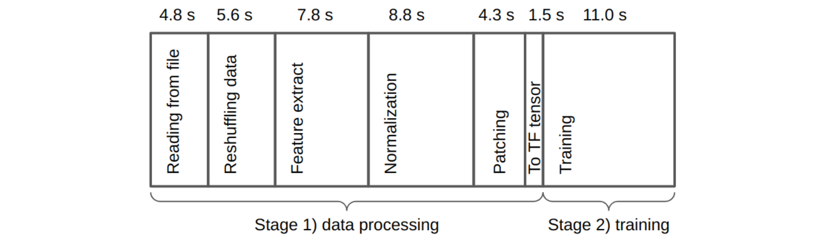
In the experiments, the data loader streams data from the disk to the GPUs. As the model is trained, the next batch of data is fetched and processed in parallel. The processing pipeline for the most expensive model (U-Net, in experiment 3) looks like this:
Diagram for typical processing and training times for one file (10GB) when training a UNET model on an A100 GPU
on Jewels-Booster. The two stages are run in parallel in a pipeline fashion. Since stage 2 is currently faster than stage 1, the
pipeline is bound by the data processing step. This is also consistent with the analysis in the Deliverable 3.4, indicating that
I/0 is still a main bottleneck for the computing performance of ML pipeline. Additionally, validation is performed after every
4th file and takes 29 seconds.
The data processing steps are done on-the-fly to allow the ML modeller the flexibility of experimenting with different data processing settings. This, however, makes the pipeline bound to the speed of the data processing, and not the training. Hence, GPU utilisation is far from optimal. We plan to alleviate this problem by parallelizing the code that performs the various data processing steps. We anticipate that with some work, the pipeline will eventually be bound by the training.
We will also investigate distributed training, by exploiting data parallelism.